Chief Minister and Minister visited MU DOT MY at NHCCE 2023–Northern Region

MU DOT MY recently concluded its participation as an exhibitor at the National Human Capital Conference & Exhibition (NHCCE) 2023 – Northern Region, organised by the Human Resource Development Corporation (HRD Corp). From May 31st to June 1st, 2023, industry leaders, HR practitioners, and professionals gathered to explore the event theme ‘HR 5.0: The Next Evolution in Human Resource Development’.

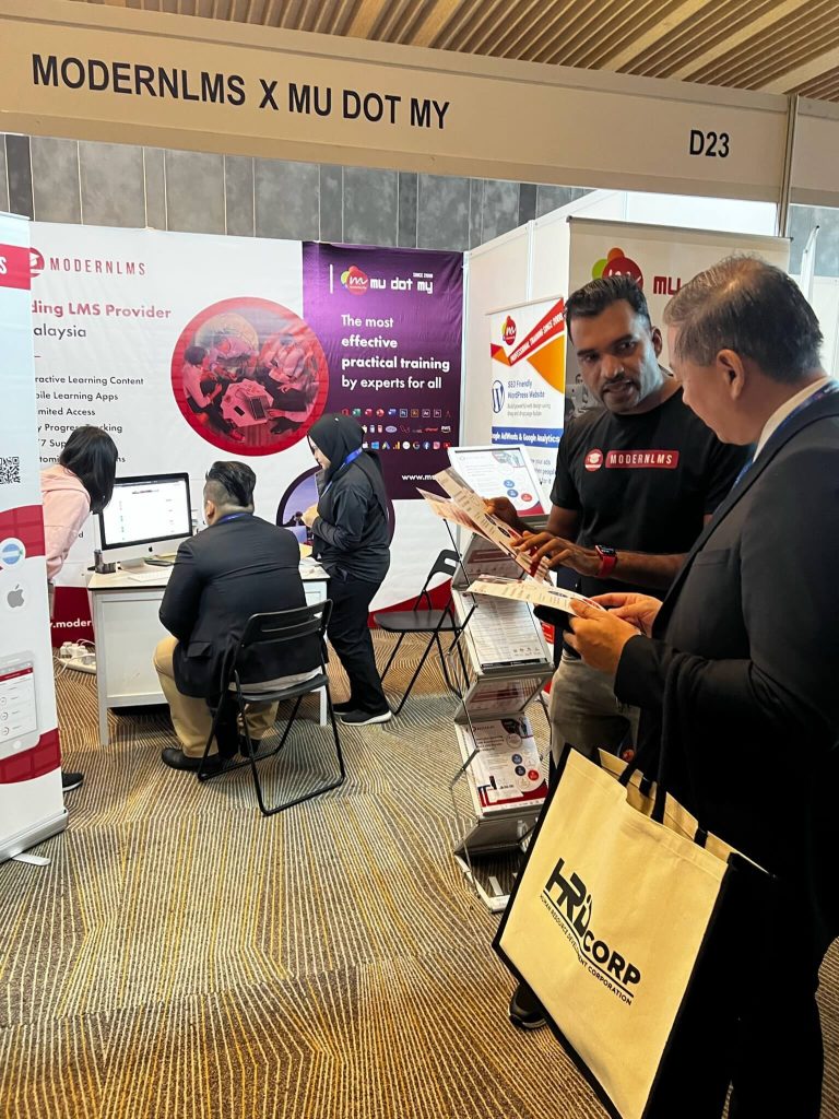
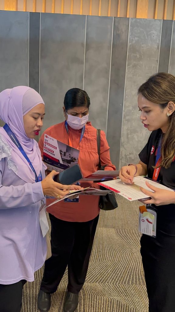
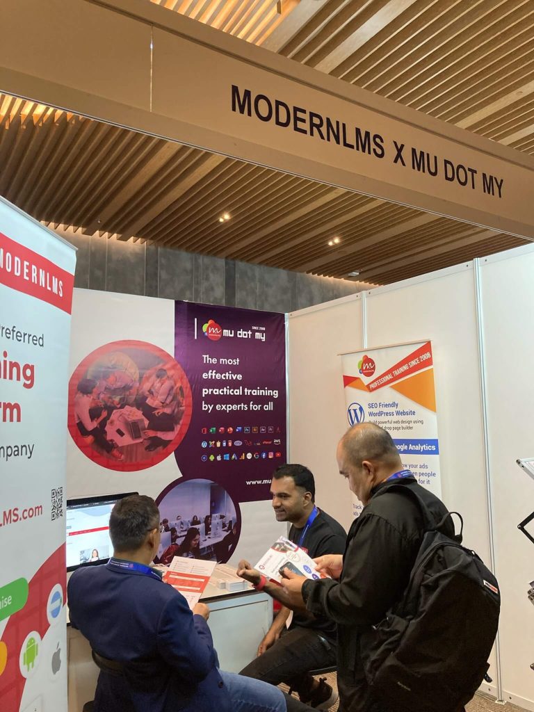
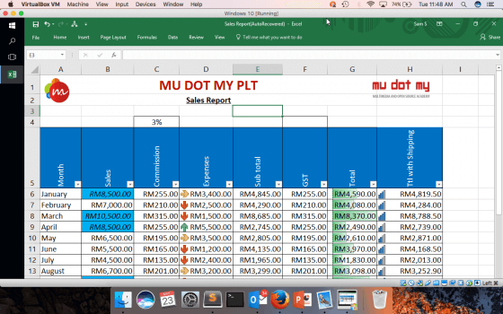
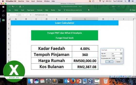
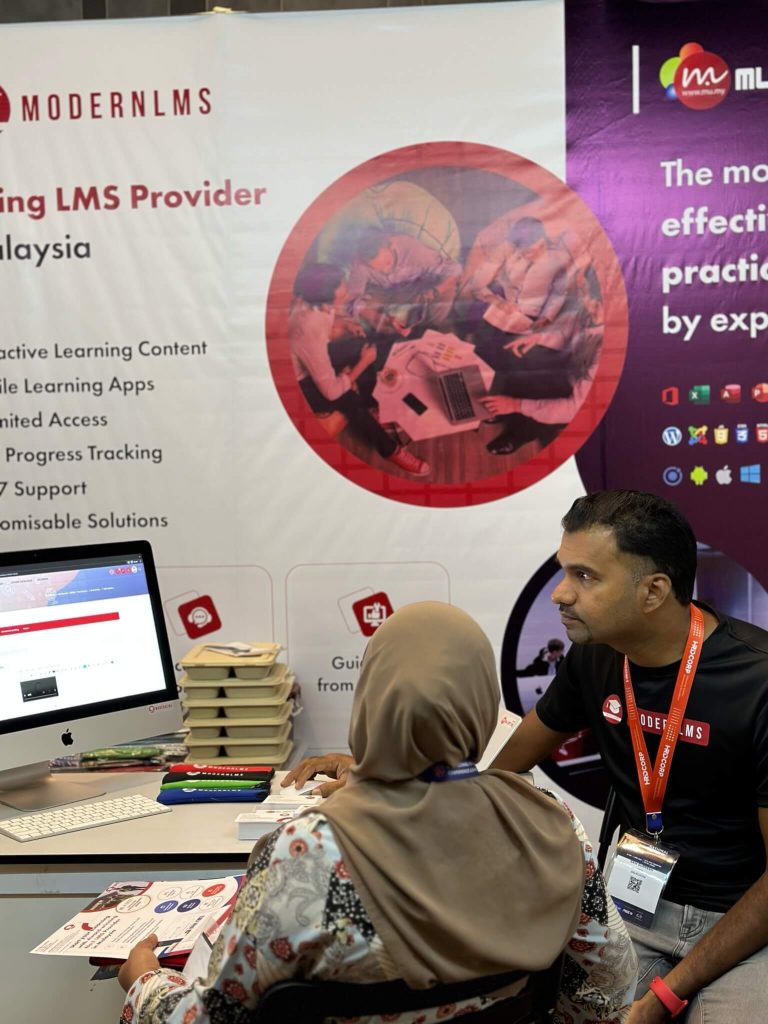
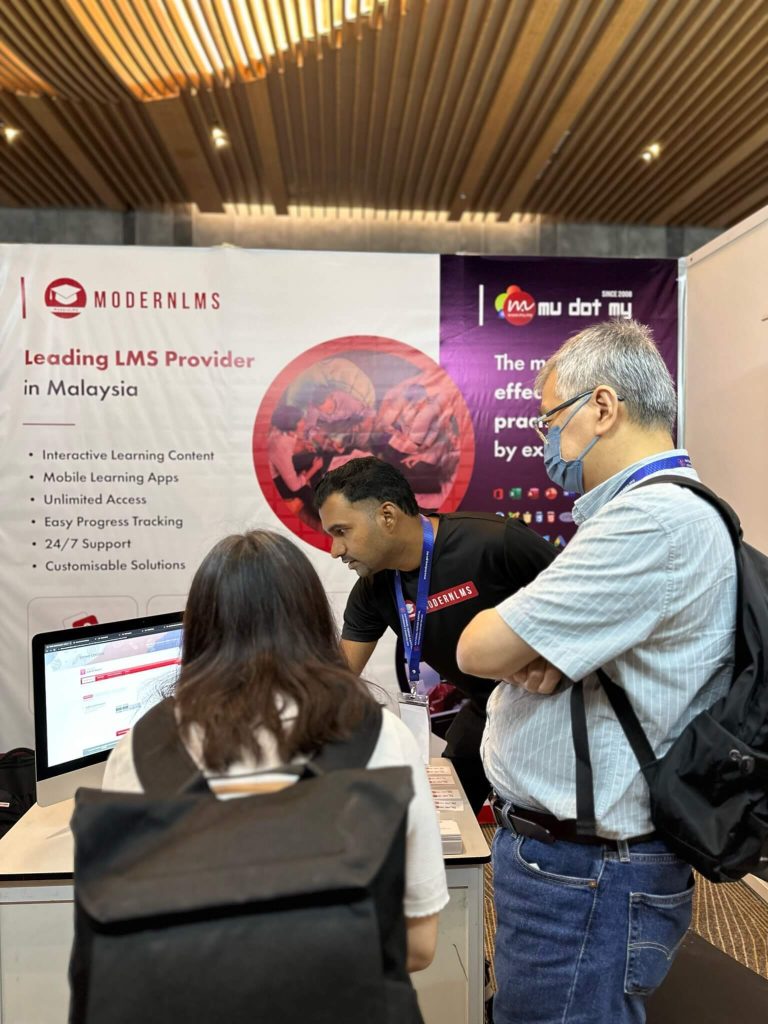
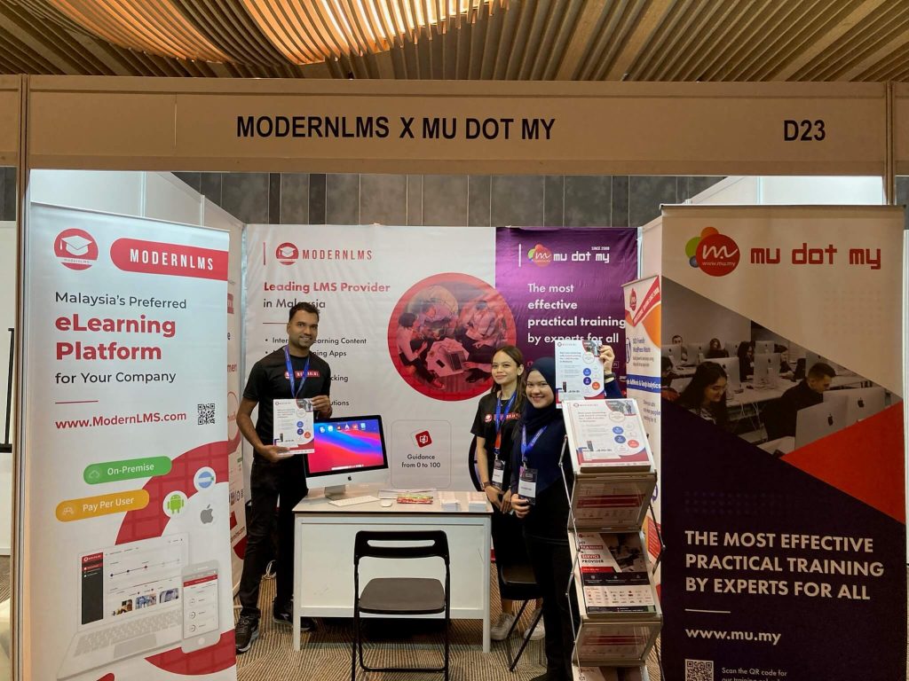
The event drew nearly 800 delegates from the northern states of Penang, Perak, Kedah, and Perlis. As one of the 50 exhibitors, MU DOT MY embraced this chance to showcase our ICT training to connect with the visitor and address their unique needs.

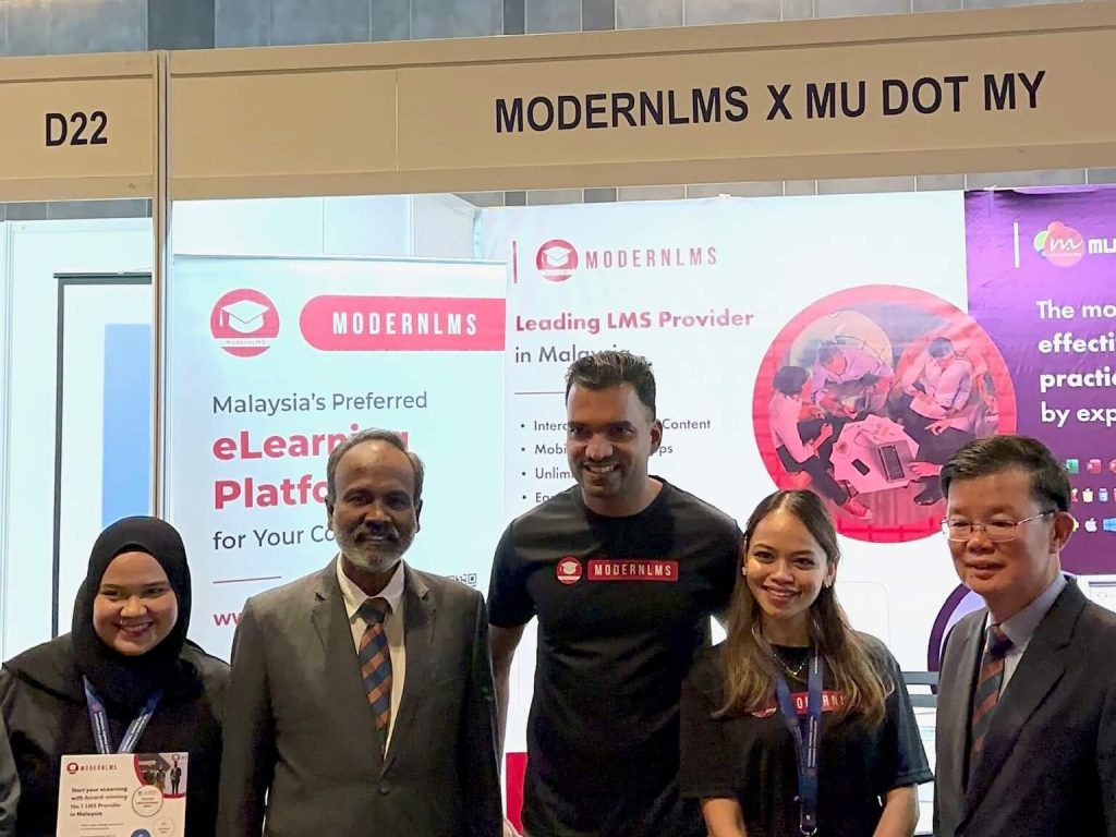
A highlight on that day was the privilege of hosting Yang Amat Berhormat Tuan Chow Kon Yeow, Chief Minister of Penang and Yang Berhormat Tuan V. Sivakumar, Minister of Human Resources at our booth. Their presence acknowledged and appreciated the contribution of our eLearning startup to the human capital landscape. It reinforced our commitment to providing innovative learning solutions and motivated us to continue pushing boundaries in the industry.

As we bid farewell to NHCCE 2023 – Northern Region, MU DOT MY eagerly anticipates the next edition of NHCCE, set to take place in Kuala Lumpur in October. We look forward to showcasing our eLearning startup’s progress, connecting with industry leaders, and exploring new avenues for collaboration and growth.

MU DOT MY ICT TRAINING

In conclusion, participating in NHCCE 2023 – Northern Region has been a memorable and rewarding experience for us. We are grateful for the opportunity. For more upcoming updates, please visit our website at https://www.mu.my/ and follow us on

Twitter: https://twitter.com/mudotmy
Facebook: https://www.facebook.com/mudotmy/

HILTI Microsoft Excel Advanced Training

On 19th April 2023, MU DOT MY conducted a Microsoft Excel Advanced Training for HILTI Malaysia. HILTI is a European company that specialises in the design and manufacture of cutting-edge technologies, software, and services for the professional construction industry.

The training was attended by 23 employees from HILTI Malaysia. During the training, the participants gained essential knowledge to unlock the full potential of Excel, explored advanced data analysis, and learned about advanced functions and pivot tables.

Our Excel Advanced course is divided into four units. Unit 1 covers advanced data entry, data tables; Unit 2 covers advanced conditional formatting and charts; Unit 3 covers lookups, while Unit 4 covers pivot tables and data relationships.

on hand practice.

Mastering Excel Advanced can help individuals and organisations improve their daily tasks’ efficiency in a simple and short-term way. At MU DOT MY, we appreciate HILTI’s commitment to global teamwork, and we are grateful for the opportunity to contribute to their growth.

excel training

If you are interested in improving your company’s efficiency, feel free to contact us to schedule your in-house Excel training!

Advanced Tips in Microsoft Excel

Why You Should Consider Using These Advanced Tips?

Some of us might have been familiar with Microsoft Excel. While others knew some basic functions or formulas. Regardless of which side you’re in, there are still many tips and tricks when using the software that we might not know, let alone be aware of their purpose. Well, fear not. In this tutorial, I will provide you with Top 10 Advanced Tips in Microsoft Excel you can apply when doing your work using Microsoft Excel.

Let's start with the advanced tips...

1. Quickly shift to the last cell in the column or row.

The first advanced tips is to quickly shift from the first cell to the last cell in the data, either from column-to-column, or row-to-row. What you have to do is simply go to the border of the cell, and then double click on the bottom border to transition to the last active cell in the column. As for shifting from row-to-row, double click on the right side of the cell border.

Shift to the last cell in the column
Shift to the last cell in the row

Bonus Tips:

You can also double click on the opposite side of the box to shift to the first cell.

2. Removing duplicates.

Removing duplication of any data becomes an easy task when using this advanced tips. You can use it to remove both words and number values.

  • First, select all the cells or data that you want to remove duplications.
  • Next, go to ribbon situated on top of the software, go to Data→Remove Duplicates.
  • Select the header for the duplicated data, and click ok.
  • A thread will be displayed once your duplication removal succeeds, click ok and you are ready to go.

3. Selecting multiple cells to insert the same data

If you plan on putting the same data or value into cells on either different cells or row, this method fits perfectly for that task.

  • First, hold the Ctrl button and select all the cells you need to put data in it.
  • Next, type in the data you need to put, and press Ctrl + Enter.

4. Autofill cells by data pattern

If you wish to insert repetitive data, such as date or months into either the whole column or row, follow these simple steps.

  • First, fill in the type of data you wanted for the column or row, for example, in the above image the data is the month.
  • Next, hover your cursor and hold the fill handle‍ – located on the lower right corner of the cell, then pull down or double click on it to fill in by column or pull it sideways to fill in by rows, until the last cell of your data.

5. Transpose data between row and column

Another advanced tips is transpose. Transpose allows you to shift your data arrangement either in row or column view. 

  • First, you have to select and copy the data you want to transpose.
  • Next, click on any blank cells that you intend to paste that data and go to Home, and select the arrow down button below the Paste option.

A number of option will pops up when you click on that button. Hover your cursor to the bottom of the pop up and click on Paste Special.

  • Once you click on Paste Special, another pop up will appear. Select transpose and click OK.

After you click OK, your data will appear in the opposite arrangement from the data you’ve selected before.

6. Wrap sentences to fit perfectly in cells

Wrap tool fits a long sentence perfectly in one cell. Simply press Alt + Enter button, or go to Home→Wrap Text and click the Wrap Text button.

7. Flash fill

Flash fill is a wonderful trick you can use which saves a lot of time when handling piles of data because it assigns the right data according to your data on the side columns.

  • Firstly, fill in the first cell with the appropriate data.
  • Next, select the next cell and press Ctrl + E.
  • Once you have hit CTRL + E, Microsoft Excel will automatically fill up the remaining blank cell with the appropriate data based on the data from the cell before it. For example, in this image, the data is month based on the date given.

Important Notes!

Flash fill only works on data in column cells.

8. Clipboard

To access clipboard in Excel, got to the Home tab and click on the button next to the word Clipboard. Your clipboard will appear on the left side of your spreadsheet.

What Do You Use Clipboards For?

When you copy anything on Microsoft Excel, the data or value that you’ve copied will be saved in the clipboard, make it easy for you to access your data there without having to scroll to find the same data. Clipboard also enables you to copy multiple data. When you want to paste it, just pick the data from your clipboard.

9. Converting a number to a money value

Need to convert numbers into money value? You can use this advanced tips to do that. Simply select the data that you want to convert, then head towards the number section under Home tab, and press button under the Number tab.

Pro Tips:

This method allows you to convert your data into almost every currency in the world.

10. Sorting data

Another interesting advanced tips that you might consider using is the sort tool. The sort tool allows us to sort raw data into organized data, either in ascending or descending order. 

  • Firstly, select the data that you need to arrange.
  • Go to the Data tab, head to the sort and filter section and click button for ascending order.
  • As for sorting the data in descending order, you must click button  and the data will sort in descending order.

Be careful!

When sorting data, some data from another cells tend to change because the data is connected to each other, and a checkbox will appear just like the one above.

11. Replace multiple same words altogether.

When handling big data that tend to change, such as a group of persons age, it must be frustating to select and change, one by one. If you opt for an easier method, you’ve come to the right place. It’s simple to change multiple words or data alltogether, actually.

  • Firstly, go to Home Tab ➜ Editing ➜ Find & Replace ➜ Replace.
  • A window will pop up. Input the words you want to replace on the first box, and on the next box, type the words that replacing it, then press   to replace all the value in the spreadsheet or to replace only one value.

Bonus Tips!

You can use the button  to find all the value mentioned written to be replaced. You can also use the button to find the value by order, from the first to the last.

12. Delete multiple error cells.

Deleting multiple errors when the spreadsheet is already finished can be done by following the steps given.

  • Firstly, go to Home Tab ➜ Editing ➜ Find & Replace ➜ Go To Special.
  • Select Formula ➜ Errors and click ok.

13. Use Macro to automate task for data of the same format

Macro is one of the advanced tips known to help user when handling a set of data, for example, financial data, which is sent to you every week. Macro helps shorten your task, while ease your daily workload too. By the way, a simple macro is no big deal, actually. You can start your very own simple macro by following the steps listed below.

  • Set up a Developer ribbon. Go to File ➜ Options ➜ Customize Ribbons and on the right side of the popup, select Developer.
  • Next, go to the Developer ribbon and click on Record Macro. A popup will appear which requires you to fill in the macro name. Press ok and start creating your procedure.
  • Once you have finished creating your procedure, and ready to save it as a macro, click Stop Recording.
  • When you want to use that macro, simply click on Macro which then a popup will appear. Select Run

Bonus Tips!

You can also start recording for macro by clicking the button situated on the bottom left corner of the software, next to the word Ready.

14. Setting Rows or Columns As Spreadsheet Guidelines

Sometimes, you might need a guideline to fill in your data, usually using the spreadsheet header, when you scroll down. You can set up a guideline by using this tip.

  • Select the header that you want to use as your guidelines, either row or column.
  • Next, go to View ➜ Freeze Panes and select Freeze Panes.

15. Using Format Painter

Format Painter is useful when you need to copy the same format of a recent table to a new table.

  • To start, first you have to select a complete table to be set as a format for your new table.
  • Go to Home and click the   button next to the Paste option.
  • When you have selected format painter, your cursor will become something like this . While your cursor is in this form, select the range of data that you want to set the format into.
  • After you’ve selected the range of data, all that’s left is to wait for Excel to transform it and once it’s done, your data will be viewed in the same format as the table you’ve selected before.

16. Impliment Cell Message Into Cells

When collaborating with others on a certain project, sometimes you want another user to avoid make changes to the cells you’ve made. To do this, you might want to put a cell message which will then pop up when someone click on the cell and display the message written on it.

  • Select the cell or range of cells that you want to display the message.
  • Head towards the ribbon, go to Data ➜ Data Tools and click the Data Validation icon on the bottom right next to Text To Column.
  • Put in your message thread into the Input message box and once you have done, click OK.
  • When the message had been set in place, your message will be displayed like this.

Conclusions

Well, that’s all this section can offer for now. Thank you for taking your time visiting and revising this section. Want to know more? Head on to our main website at https://www.mu.my/en/, and register for our course training to know more about Microsoft Excel Tips. We also provided bonus formulas and functions for those who attend this course training.

Other Post You Might've Interested

Microsoft Excel Shortcuts That You Should Know

How many shortcuts do you know for Microsoft Excel?

Learn these useful Excel shortcuts to save your time working on spreadsheets.

Learn more at www.mu.my

What is a PivotTable?

PivotTable is one of the most powerful features in Excel. It will save you a lot of time to summarize your large, detailed data set into a meaningful report.

Read more

Conditional Formatting in Excel

Make your data easier to read.

With Conditional Formatting, you can highlight the data with a certain colour or style based on cell values. For example, you can highlight the sales above RM8000 by creating a certain rule. You also can find duplicated items, hide errors, compare two lists, etc. Conditional Formatting is a powerful feature and can do more than many people realize.

Want to learn more on Conditional Formatting in Excel, enroll with us http://excel.my/

Upcoming Excel Training Basic to Advance on 13-14 July 2017.
Contact info@mu.my or 03-80116639.
Find out more at https://www.mu.my/

Goal Seek in Excel

Situation: You want to buy a house and the lender offers loan on at RM 500,000 over 20 years. With this, you can find out how much your payback per month using all those calculators on the net.

However, what if you set your budget to pay RM 1,300 instalment per month? So based on mortgage rate, how much worth of house you can afford for RM 1,300 per month?

Goal Seek allows you to analyses the best value for you to achieve your desired goal.

Want to learn more about Goal Seek in Excel, enrol with us http://www.excel.my/

Upcoming Excel Basic to Advance on 7-8 June and 13-14 July 2017.

Contact info@mu.my or 03-80116639.

Find out more at https://www.mu.my